Patch antenna
Description
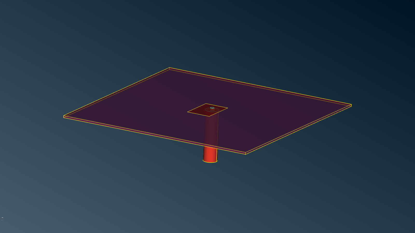
This model, inspired from [1], is made of a coaxial waveguide feeding a patch antenna on a lossy dielectric substract.
We wish to compute radiation diagrams as well as the reflection coefficient around the resonance frequency about 5.02 GHz.
The PSHELL of the model are named after its different objects.
Volumic domains
In this model there are three homogeneous volumic dielectric domains:
SUBSTRACT: the substract on which the metallic patch is printedGUIDE: the coaxial waveguideEXT: the exterior domain (unbounded)
There is one perfect volumic metallic domain:
CORE: the core of the coaxial waveguide
Surfacic interfaces
The gain is the perfect conducting (PEC) metallization between the waveguide and the exterior domain:
GUIDE/EXTinterface
There are PEC metallizations between the substract and the exterior domain:
the ground
the patch
There are dielectric interfaces between:
the substract and the exterior domain
the waveguide and the substract
There are interfaces between dielectric and perfect metallic domains:
the core and the waveguide
the core and the substract
the core and the exterior domain
Modal Surface
The coaxial modal surface is used to model a semi-infinite adapted waveguide. It is used to illuminate the coaxial transmission line by its TEM mode.
download
patch-coax.ansa.gz (ansa v24.0.0)
CAD and Mesh tips
Waveguide
It is important to ensure that the length of the waveguide is not too small compared to the wavelength in the waveguide domain. In this model it is about half of the largest wavelength.
One has to imagine that the modal surface is the interface to a semi-infinite domain. Hence the end of the core next to the modal surface is not a metallic/dielectric interface and must be ignored.
Mesh rules
The mesh is globally set to be equal to approximately \(\lambda/10\) in the dielectric domain. It is refined:
on the modal surface for a good representation of the TEM mode
around patch border where the current can vary rapidly
around ground and substract singularties
Simulation setup
Physical properties
You can use the following values for relative permittivity and permeability of the volumic domains:
Name |
\(\varepsilon'\) |
\(\varepsilon''\) |
\(\mu'\) |
\(\mu''\) |
|---|---|---|---|---|
air |
1.0 |
0.0 |
1.0 |
0.0 |
substract |
4.34 |
0.08681 |
1.0 |
0.0 |
waveguide |
2.2 |
0.0 |
1.0 |
0.0 |
Warning
ASERIS works in \(e^{-i\omega t}\) time convention. Hence imaginary part of lossy materials must be positive.
Illumination
The coaxial transmission line is illuminated by its first TEM mode.
We consider a frequency sweep around 5.02 GHz from 4.92 GHz to 5.12 GHz with a step of 20MHz.
Observation
We wish to compute the radiation pattern for all directions, that is for \(\theta\) in [-180° 180°] and \(\phi\) in [0 180°], with an angular step of 3°.
We can also access the reflection coefficient inside the modal surface.
Results
Below are some representations of the solution in terms of current density, far field diagram and reflection coefficient.
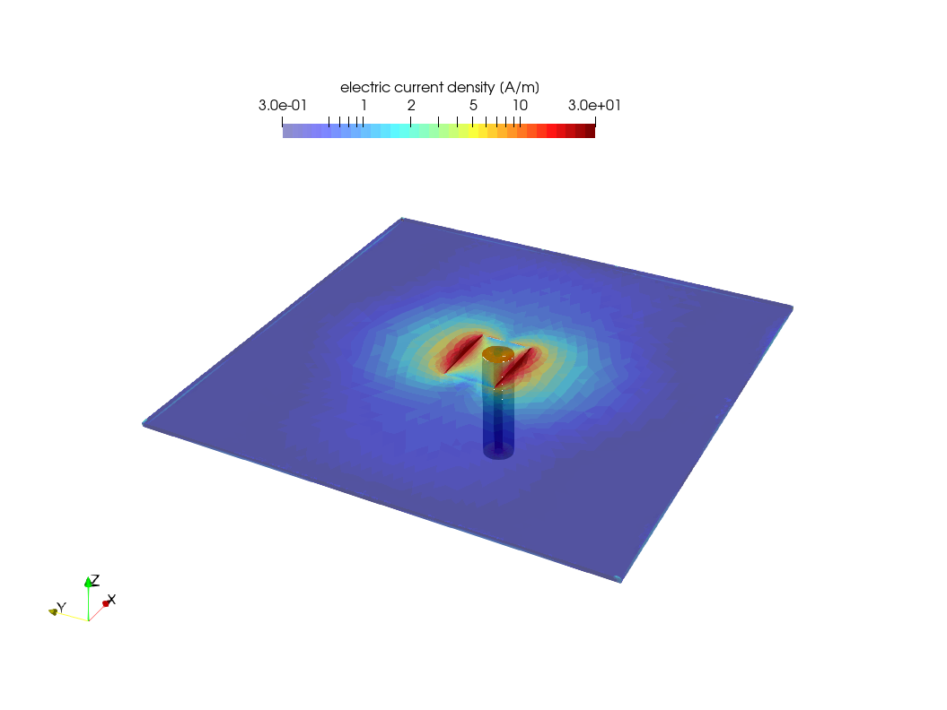
Current density at 5.02GHz. One can see the patch resonance at patch border. The waveguide is visible by transparency.
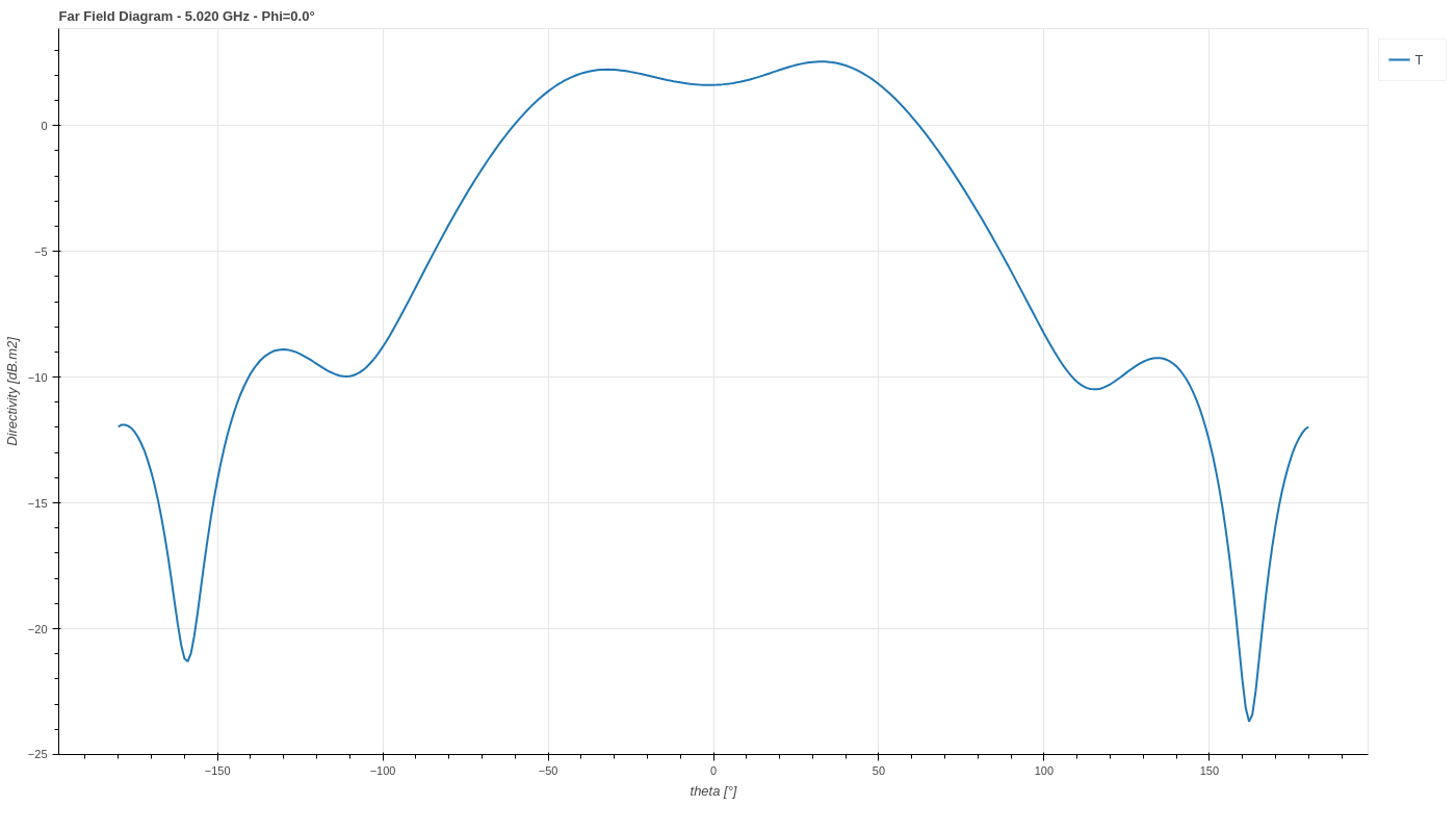
Directivity diagram of the total far field at 5.02 GHz. While the far field has been computed for all frequencies and all directions, one can draw slices for fixed angles, e.g. here at \(\phi=0\) °.
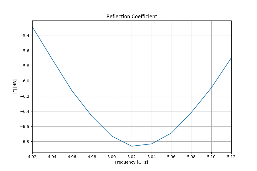
Reflection coefficient. The minimum is obtained around 5.02 GHz.