Theoretical foundations
ASERIS-BE
ASERIS-BE uses the Boundary Element Method (BEM) to solve the time-harmonic Maxwell’s equations for a wide range of electromagnetic applications, spanning from DC to high frequencies. It incorporates sophisticated parallel and out-of-core fast linear solvers, including the multi-level Fast Multipole Method (FMM) and the H-matrix method. This document outlines the theoretical principles underlying the software.
Maxwell’s equations
ASERIS-BE solves the 3D Maxwell’s equations in the frequency domain with some radiation conditions. For a more complete presentation, we first introduce the equations in the time domain.
Hereafter, \(\Omega\) represents a domain in \(\mathbb R^3\).
Maxwell’s equations in the time domain
The time domain Maxwell equations in \(\Omega\) are written as follow:
where
\(\vec e(\mathbf {r}, t)\) is the electric field;
\(\vec d(\mathbf {r}, t)\) is the electric displacement;
\(\vec h(\mathbf {r}, t)\) is the magnetic field;
\(\vec b(\mathbf {r}, t)\) is the magnetic induction;
\(\vec j_s(\mathbf {r}, t)\) is the electric current density;
\(\vec m_s(\mathbf {r}, t)\) is the magnetic current density.
Linear constitutive relations
\(\vec e\), \(\vec d\), \(\vec h\) and \(\vec b\) are related by the so-called constitutive relations. We only consider linear relations of the form:
and
where
\(\varepsilon(\mathbf {r}, t)\) is the local electric permittivity;
\(\mu(\mathbf {r}, t)\) the local magnetic permeability;
These relations are assumed to be causal, which means
In the vacuum, these properties are uniform and instantaneous:
\(\varepsilon_0 = 8.85418782 \ldots 10^{-12} \rm F m^{-1}\) is the vacuum permittivity and \(\mu_0 = 4\pi\times 10^{-7} = 1.25663706 \ldots 10^{-6} \rm H \, m^{-1}\) is the vacuum permeability.
Wave propagation
In homogeneous, non-dispersive media, i.e. if
a simple calculation shows that the electric and magnectic fields are solutions to the homogeneous vector wave equations
outside source regions, with the propagation celerity c
We denote by \(c_0\) the celerity of light in vacuum:
Example of electromagnetic wave
Plane waves represent the prototype of electromagnetic waves. Given a real-valued function \(g(t)\), two vectors \(\vec E_0\) and \(\vec H_0 \in \mathbb R^3\) and a unit vector \(\hat \nu \in \mathbb R^3\), the fields
define progressive waveguides propagating in vacuum without attenuation or distortion in the direction \(\hat \nu\). They are exact solutions of homogeneous Maxwell’s equations in the free space (vacuum):
if and only if
\(Z_0 \approx 376.730313461 \, \Omega \; (\rm Ohm)\) is called the vacuum characteristic impedance.
Time-Harmonic dependence convention of \(e^{-i\omega t}\)
If \(u(t)\) is a real-valued function of the time variable, we define its Fourier transform \(U(\omega)\) as
where \(\omega\) is the angular frequency (in \(\rm rad. s^{-1}\)), \(\omega = 2\pi f\), and \(f\) the frequency (in \(\rm Hz\)). Furthermore, it is important to note that \(U(-\omega) = \overline{U(\omega)}\) for all \(\omega \in \mathbb R\), thus considering only positive frequencies is sufficient.
The inverse Fourier transform allows to go back to the time domain:
ASERIS-BE uses the \(\textcolor{red}{ e^{-i\omega t}}\) time-harmonic convention
All input data are assumed to follow this convention, and correspondingly, all output data adhere to the same convention.
Important
Note that adopting the opposite convention results in complex conjugate fields and currents.
Warning
Mixing conventions in the simulation workflow can lead to erroneous results.
Time harmonic Maxwell’s equations
where
\(\vec E(\mathbf {r}, \omega)\) is the electric field;
\(\vec H(\mathbf {r}, \omega)\) is the magnetic field;
\(\varepsilon(\mathbf{r},\omega)\) is the local electric permittivity;
\(\mu(\mathbf{r}, \omega)\) the local magnetic permeability;
\(\vec J_s(\mathbf{r}, \omega)\) is the electric current density;
\(\vec M_s(\mathbf {r}, \omega)\) is the magnetic current density.
To simplify notations, we used the same symbols to represent permittivity and permeability in both the time and frequency domains without causing confusion.
Reduced wave equation or Helmholtz equation
In homogeneous media, i.e.
a straightforward calculation shows that the electric and magnetic fields are solutions to the homogeneous vector reduced wave equation, aka the Helmholtz equation
outside source regions, with
Time harmonic plane waves have the following expression:
where
and \(\vec E_0(\omega)\) and \(\vec H_0(\omega)\) are complex-valued 3D-vector satisfying:
If \(\mathbf k \in \mathbb R^3\), the plane wave is periodic in the direction \(\hat \nu\) with period \(\lambda\).
3D-domains
In ASERIS-BE, we deal with piecewise homogenous media. A homogeneous volumic material \(\Omega\) is characterised by its relative electric permittivity \(\varepsilon_{r} = \varepsilon/\varepsilon_{0}\) (unitless) and its relative magnetic permeability \(\mu_{r} = \mu/\mu_{0}\) (unitless).
These characteristic parameters are given in the frequency (complex numbers):
The celerity in the domain \(\Omega\) is given by
The characteristic impedance of the domain is given by
3D-conductors
ASERIS-BE handles perfect conductors or Perfect Electric Conductors (PEC). There is no need to solve Maxwell’s equations in such domain: total electromagnetic field is identically zero.
A 3D material may have a finite conductivity. In such cases, it is characterised not only by its relative electric permittivity \(\varepsilon_{r}\) and relative magnetic permeability \(\mu_{r}\), but also its electric conductivity \(\sigma\) (in \(\rm S \, m^{-1}\)).
Within this domain, Ohm’s law states that
Exterior domain
We refer to the exterior domain as the complement of some bounded domain in \(\mathbb R^3\). Typically, within this domain \(\varepsilon=\varepsilon_0\) and \(\mu=\mu_0\), yet users have the flexibility to impose any complex values.
Causality & Radiation condition
In the time domain, we assume causality: if sources are zero for negative times \(t<0\) then electric and magnetic fields should also be zero for negative times. In the frequency domain (i.e. for time-harmonic solutions), time variable is absent and the frequency variable acts as a fixed parameter: we solve a different and independent PDE for each frequency. The causality condition is substituted with a requirement concerning the solution’s behavior “at infinity”, known as the radiation condition.
A scalar solution \(u\) of the Helmholtz equation should satisfy the Sommerfeld outgoing radiation condition at infinity:
Each component of the electric and magnetic fields satisfies this condition.
Yet, the electric and magnetic fields not only satisfy the Helmholtz equation but also have their components related to each other through the Maxwell equations. The radiation condition can thus be reformulated more suitably as the Silver-Müller radiation condition:
where \(\hat{r} =\mathbf{r}/r\). It states that when moving towards infinity in a direction \(\hat r\), the EM wave must exhibit behavior akin to a plane wave propagating in that specific direction
Integral representation theorem
Integral representation formula, aka Stratton-Chu formula
Let’s consider a homogeneous domain \(\Omega\) which can be either bounded or an exterior domain. It is characterised by \(\varepsilon\) and \(\mu\). We denote by \(\Gamma = \partial \Omega\) its boundary. \(\hat n\) is the unit outward normal on \(\Gamma\).
If \((\vec E, \vec H)\) is an electromagnetic field satisfying the homogeneous time-harmonic Maxwell equations (i.e. without current sources in the right-hand-side) and the Silver-Müller radiation condition at infinity (if \(\Omega\) is an exterior domain) then for all \(\mathbf r \in \Omega\):
where
\(\displaystyle k = \frac{\omega}{c}\) is the wavenumber;
\(\displaystyle G(\mathbf r, \mathbf r') = \frac{e^{ik|\mathbf r - \mathbf r'|}}{4\pi |\mathbf r - \mathbf r'|}\) is the Helmholtz Green’s kernel satisfying the Sommerfeld radiation condition;
\(\vec j = \vec H \times \hat n\) is the equivalent electric surface current density on \(\Gamma\);
\(\vec m = -\vec E \times \hat n\) is the equivalent magnetic surface current density on \(\Gamma\).
Note
For \(\mathbf r \in \Omega' = \mathbb R^3 \setminus \Omega\), the integral representation formulas lead to zeros electric and magnetic fields.
For \(\mathbf r \in \Gamma\), the tangential components have the following representation:
where \(\Pi_{\mathbf r} \vec u (\mathbf r) = \vec u_\parallel (\mathbf r)= - \hat n \times ( \hat n \times \vec u )\) is the tangential projection of a given vector field \(\vec u\) on \(\Gamma\) at point \(\mathbf r \in \Gamma\).
Note
Note that for any given surface current densities \(\vec j\) and \(\vec m\), the integral representation formulas define an electromagnetic field \((\vec E, \vec H)\) which satisfies the homogeneous Maxwell equations and the Silver-Müller radiation condition at infinity.
Note
The therorem can be generalised to take into account the presence of open, non-manifold surfaces and thin wires.
Important
In ASERIS-BE, we look for electromagnetic field in this form within each homogeneous domain. The unknowns are not the electric and magnetic fields themselves, but rather the electric and magnetic equivalent surface current densities on the boundaries and interfaces between homogeneous domains. Thus Maxwell’s equations and radiation conditions are exactly satisfied. The only approximation arises in fulfilling the boundary and transmission conditions.
Boundary conditions
Supported materials, models, sources and boundary conditions.
Boundary conditions
On the boundary \(\Gamma_{\rm PEC}\) of a perfect Electric Conductor (PEC), we impose the following boundary condition:
On the boundary \(\Gamma_{I}\) of an impenetrable objet representing an imperfectly conducting or treated body, we impose an impedance boundary condition:
where \(Z_s\) is the surface impedance in \(\Omega\) (also referred to having units \(\Omega / \square\), Ohm-per-square). On a thin sheet, this surface impedance may be different on each side of the surface (+ or -). ASERIS-BE takes into account this kind of dual impedance boundary condition (\(Z_s^+, Z_s^-\)).
Note
Orientation of the surface matters in case of dual impedance.
Interface conditions
Tangential components of electric and magnetic fields are continuous across the interface between two adjacent dielectric domains \(\Omega_i\) and \(\Omega_j\):
where \([\cdot]\) represents the jump across \(\Gamma_{i,j}\).
Thin resistive sheets \(\Gamma_{R}\) can be modeled by using a general transmission impedance condition:
For example, in the low frequency regime, a thin conductor, characterised by its thickness, conductivity and permittivity (\(d, \sigma, \varepsilon)\) may be modeled by
Wires
ASERIS-BE integrates a thin wire model allowing to represent only the neutral axis of the beam. It is meshed using linear segments. Thin wires may be characterised by their radius \(a\), and their lineic resistance, inductance and capacitance values (\(R, L, C\)), or alternatively their lineic impedance. The model also handles dielectric coating.
Local values
Local values can be used to model (small) equipements. They are generally positioned on a wire or at the junction of a wire and a (perfectly or imperfectly) conducting surface.
Lumped elements: local impedance \(Z_c\), any complex number or (R, L, C) circuit
Voltage generators
Ports
Sources
ASERIS-BE implements differents types of sources:
Voltage generators (generally on wires).
Point sources:
electric and magnetic dipole sources,
directive sources (characterised by a farfield diagram).
Incident modes on modal surfaces:
rectangular waveguides: TE/TM modes,
coaxial waveguides: TEM mode.
Incident plane waves characterised by the direction of arrival \(-\hat \nu\), i.e. the opposite of the direction of propagation, and V/H polarisations.
Binary file providing directly the right-hand-side (RHS) for the solver. This kind of source is used in coupling problems.
Ground plane and symmetries
Geometric symmetries and infinite ground plane (PEC surface) are handled by ASERIS-BE.
Possible planes are \(X=0\), \(Y=0\) or \(Z=0\).
Note
A maximum of 2 symmetry planes can be handled simultaneously. That allows to mesh a half or a quarter of the studied object.
Note
Only 1 ground plane can be defined in a model (without any additional geometrical symmetry plane).
Integral Equations
To solve a general Maxwell’s equations problem - i.e. PDE system with boundary and transmission conditions, along with radiation condition at infinity- we look for electromagnetic field using an integral representation within each homogeneous domain. This representation utilizes the electric and magnetic equivalent surface current densities on the boundaries and interfaces between these domains as the unknowns. Integral equations are derived by satisfying the boundary and transmission conditions on all boundaries and interfaces.
To illustrate the general procedure, let’s consider the example of a bounded PEC object \(\Omega_0\) illuminated by an incident plane wave \((\vec{E}^{in}, \vec{H}^{in})\). Here, \(\Omega = \mathbb{R}^3 \setminus \overline{\Omega_0}\) represents the complementary exterior domain assumed to possess vacuum properties. Additionally, \(\Gamma = \partial \Omega\) denotes its boundary, and \(\hat{n}\) represents the unit outward normal.
The integral representation theorem allows us to look for the electric field in the form:
for any \(\mathbf r \in \Omega\). Magnetic surface current density is zero: \(\vec{m} = \hat n \times \vec{E} = \vec 0\).
The integral equation is obtained by imposing the boundary condition, i.e. for all \(\mathbf r \in \Gamma\):
or, in other words, we look for a tangential current \(\vec j\) defined on \(\Gamma\), such that for all \(\mathbf r \in \Gamma\)
This is the Electric Field Integral Equation (EFIE). It can equivalently be formulated using the Rumsey reaction principle: find \(\vec j\) in some functional space \(V\) of admissible tangential currents, such that for all \(\vec j^t \in V\):
This is the variational formulation of the EFIE. \(V=\text{TH}^{-1/2}(\rm div, \Gamma)\) is the natural variational space: the space of tangential currents in \(\text{TH}^{-1/2}(\Gamma)\) whose tangential divergence are in \(\text{H}^{-1/2}(\Gamma)\).
Boundary Element Method (BEM)
ASERIS-BE is based on the Boundary Element Method, a Galerkin approximation technique involving the approximation of space \(V\) with a finite-dimensional space \(V_h\). It solves the subsequent variational formulation: find \(\vec{j}_h \in V_h\), such that for all \(\vec{j}^t \in V_h\):
where \(\Gamma_h\) is a piecewise linear approximation of \(\Gamma\) achieved through a triangular mesh, \(V_h\) is a finite-dimensional subspace of \({\rm TH}^{-1/2}({\rm div}, \Gamma_h)\) of piecewise tangential affine currents.
The first order Raviart-Thomas \(H(\rm div)\) Finite Element
The finite element is defined by the triplet \((T, {\mathcal V}, {\mathcal L})\):
the reference element \(T\) is a triangle \((S_1S_2S_3)\):
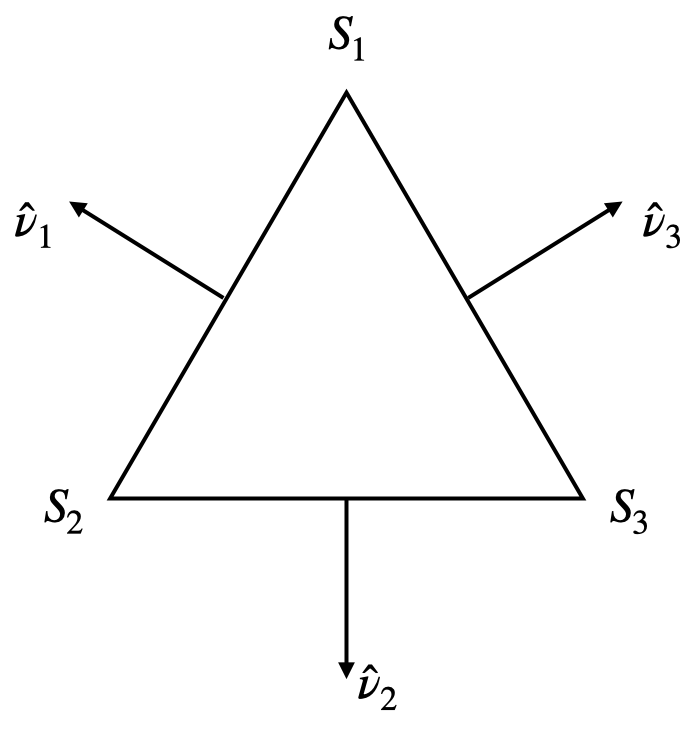
Reference triangle \(T=(S_1S_2S_3)\). \(\hat \nu_i\) represents the outward unit normal on edge \(a_i = [S_i, S_{i+1}]\) (operation + modulo 3).
\({\mathcal V}\) is the space of polynomial tangential vector fields on \(T\) defined by:
\[{\mathcal V} = \{\vec w(\mathbf r) = \vec \alpha_T + \beta_T \mathbf r, \; \text{for } \mathbf r \in T, \; \vec{\alpha}_T \in \mathbb C^2, \beta_T \in \mathbb C\}`\]\(\rm dim \, \mathcal V = 3\). Note that \(\rm div_T \vec w \mathbf r)= 2 \beta_T\) for \(\mathbf r \in T\).
\({\mathcal L} = \{l_1, l_2,l_3\}\) is the basis of the dual space \(\mathcal V^*\) of linear forms
\[l_i(\vec w) = \int_{a_i} \vec w (\mathbf r) \cdot \hat \nu_i da_i\]\(l_1, l_2,l_3\) are called the degrees of freedom in the reference element (local DoF’s).
\(H(\rm div^1)\) Basis function
In the reference element \(T\), we define the basis functions \((\vec w_1, \vec w_2, \vec w_3)\) as follows:
where \(|T|\) is the area of triangle \(T\). They satisfy the relations:
These basis functions are sometimes referred to as the Rao-Wilton-Glisson (RWG) basis functions.
A function \(\vec{j}^t \in V_h\) is defined by its degrees of freedom: on an edge \(a\) connecting two triangles \(T\) and \(T'\), the outgoing flux from \(T\) should be equal to the incoming flux into \(T'\).
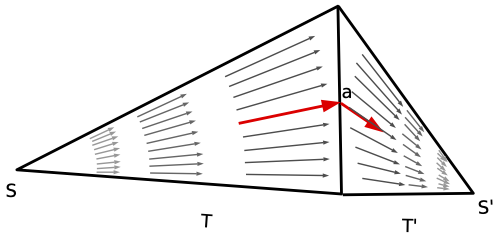
First order Raviart-Thomas basis function associated with edge \(a\) oriented from \(T\) to \(T'\).
Note
These definitions can be generalised to 1D-beam elements (or segment). Current density on a beam element is picewise vector aligned with the segment. It takes into account the radius \(r\) via a factor \(2 \pi r\). DoF are defined as the flux at endpoints across their circular section, and hence have the same status as DoFs on triangles.
Orientation - multiple junctions & free edges
The global DoFs definition depends on an arbitrary orientation of edges and endpoint of segments: \(\hat \nu\) the direction of the current flow. Generically, a DoF “connects” 2 elements and represents the current flowing from one element to the other.
ASERIS preprocessor analyses the information-enriched BEM mesh and construct the finite element model. It handles multiple junctions (several DoFs on the same edge) and free edges (no DoF).
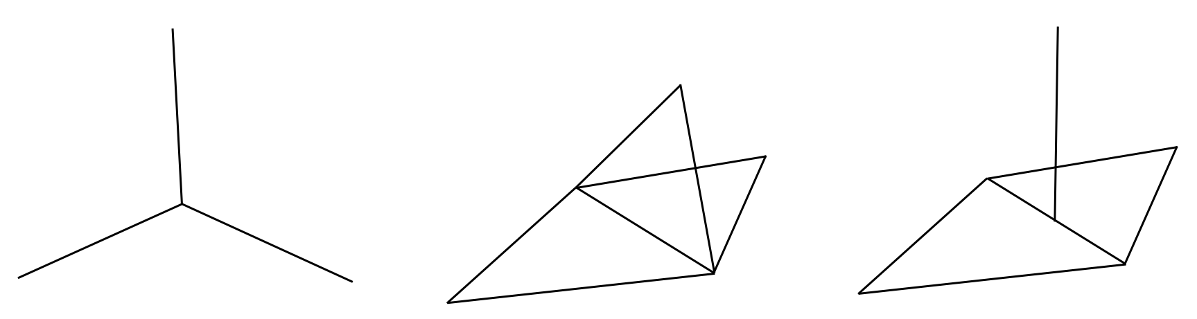
Example of multiple (triple) junctions: between wires (left); between triangles (center); between wires and triangles (right)
The number of DoFs is roughly equal to the number of triangle edges and segments vectices in the mesh.
Solvers
Linear system
If \(N\) is the number of degrees of freedom, looking for the unknown current \(\vec j_h\) in the form of
and using \(\vec j^t_h = \vec w_i\) for \(i=1, \ldots, N\) in the testing procedure, we obtain the following linear system:
where
\(\mathbb Z\) is the impedance matrix:
\[\mathbb{Z}_{ij} = ikZ_0\left( \int_{\Gamma_h\times \Gamma_h} G(\mathbf r, \mathbf r') \vec w_j (\mathbf r') \cdot \vec w_i (\mathbf r) d\Gamma_h(\mathbf r') d\Gamma_h(\mathbf r) -\frac{1}{k^2} \int_{\Gamma_h \times \Gamma_h} G(\mathbf r, \mathbf r') {\rm div}_\Gamma \vec w_j (\mathbf r') {\rm div}_\Gamma \vec w_i (\mathbf r ) d\Gamma_h(\mathbf r') d\Gamma_h(\mathbf r) \right)\]and it indeed has the dimension of an impedance (in \(\Omega\)).
\(I\) is the unkown vector of degrees of freedom:
\[I = (I_1, \ldots, I_N )^T\]It has the dimension of a current (in \(A\)).
the right-hand-side (RHS) \(\mathbb U\) represents the incident electric field tested across mesh edges
\[\mathbb U_i = - \int_{\Gamma_h} \vec E^{in} (\mathbf r)\cdot \vec w_i (\mathbf r)d\Gamma_h(\mathbf r)\]It has the dimension of a voltage (in \(V\)).
Note
\(\mathbb Z\) is a full complex symmetric (non Hermitian) matrix. Its elements involve evaluating singular integrals over pairs of triangles.
Note
A classical matrix assembling procedure requires \(O(N^2)\) floating-point operations, and \(O(N^2)\) bytes to store the matrix.
Note
A classical direct method resolution, such as Gauss or Cholesky factorization, requires \(O(N^3)\) floating-point operations.
Important
This quickly becomes limiting in terms of memory and CPU capacity. Hence the need for advanced fast solvers.
Advanced solvers
The use of fast algorithms and HPC (High-Performance Computing) is essential for implementing simulations in industrial applications.
The Fast Multipole Method (FMM) coupled with iterative solvers [Greengard1987]:
Matrix-vector product in \(O(N \log N)\) operations.
Efficient HPC implementation [Sylvand2002].
Challenges: low frequencies or locally refined meshes, poor conditioning, a large number of right-hand sides (RHS)…
H-Matrix direct solver [Hackbusch1999] [Hackbusch2000]:
\(O(N \log^2 N)\) complexity demonstrated for kernels with asymptotically regular behavior (such as the Laplacian kernel).
Recent efficient parallel implementations and solid theoretical foundations for oscillating kernels [Lize2014] [Delamotte2016].
Fast Solvers: General principles
Fast methods are generally based on the possibility of a low-rank approximation of the Green’s kernel. For example, let’s consider for two point cloudw \((\mathbf{x}_i)_{1 \le i \le m}\) and \((\mathbf{y}_j)_{1 \le j \le n }\) in \(\mathbb R^3\), the \(m \times n\) matrix:
Under some conditions of separation of these two clouds, it can be demonstrated that this matrix has a low rank approximation:
with \(U \in \mathbb C^{m \times r}, \; V \in \mathbb C^{n \times r}\), \(r \ll m, \, n\). \(G_r = U V^T\) is the compressed approximation of \(G\).
Consequences:
Reduced storage: it takes \(O((m+n)r)\) bytes to store \(U\) and \(V\) instead of \(O(mn)\) for \(G\).
Accelerated interaction computations: for example, if \(q \in \mathbb C^n\), the matrix-by-vector product \(V = G q\) can performed with \(O((m+n)r)\) floating-point operations instead of \(O(mn)\) operations.
This kind of compression can be achieved either analytically or by algebraic means. For example, if we could find an expansion of the kernel in the form:
then \(U_{i,l} = g_l(\mathbf{x}_i)\) and \(V_{j,l} =h_l(\mathbf{y}_j)\) provide a low-rank approximation of \(G\).
FMM
Such an expansion is used in the Fast Multipole algorithm.

Two separated clusters. We set: \(\mathbf{r}_{12} = \overrightarrow{M_1M_2}\) and \({r}_{12} = M_1M_2\).
The Gegenbauer formula asserts that:
with
Here \(S^2\) represents the unit sphere, \(h_l^{(1)}\) the Hankel function of the first kind and \(P_l\) the Legendre polynomial of degree \(l\).
A low rank approximation can be achieved by appropriately choosing \(L\) and discretising the integral on the unit sphere.
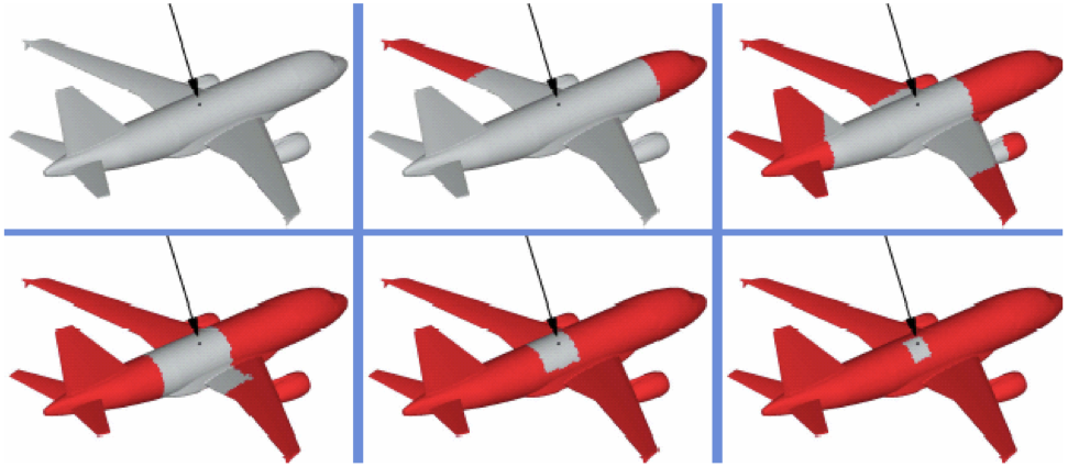
The general multilevel procedure is a divide and conquer algorithm based on an octree decomposition and the recursive application of FMM interaction between non-neighboring cells. Classical interactions are used for neighboring leaves.
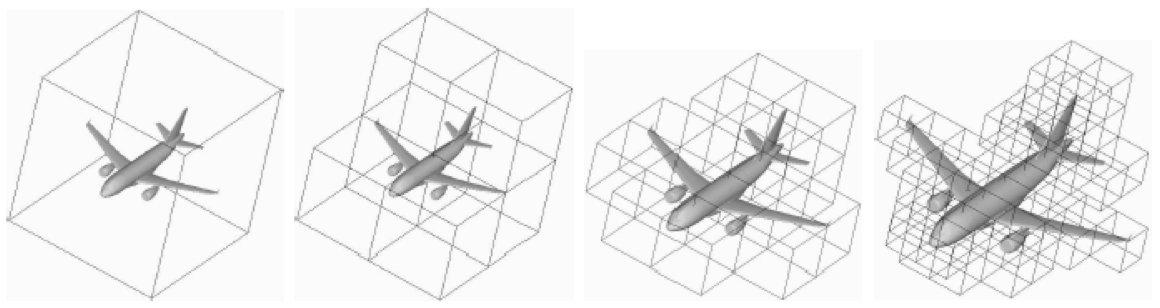
Example of octree decomposition.
Neighbors vs Non-neighbors.
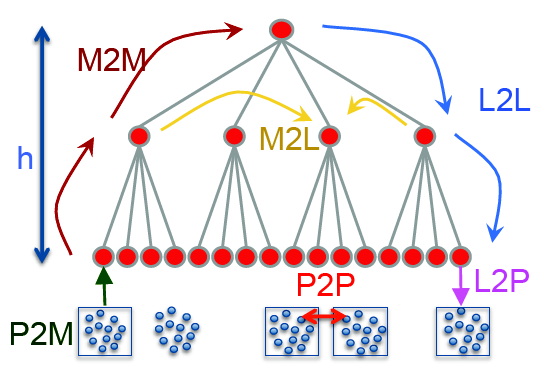
FMM algorithm.
This procedure allows a fast matrix-by-vector product computation: in \(O(N \log N)\) floating-point operations instead of \(O(N^2)\). To solve the linear system \(\mathbb{Z} I = \mathbb{U}\), an iterative method is used along with a preconditioner. ASERIS-BE implements a SPAI preconditioned GMRES algorithm.
H-Matrix
H-matrix provides another systematic compression method that allows to assemble a compressed approximation of \(\mathbb Z\) matrix, perform a compressed Cholesky decomposition and solve the system. It is also based on a hierarchical space decomposition, referred to as clustering.
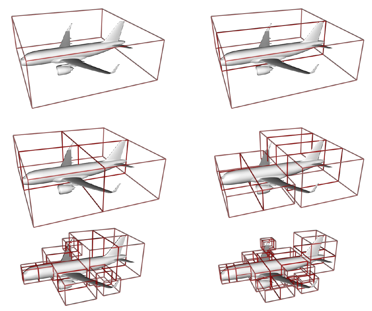
Bisection based cluster tree.
The second ingredient is an admissibility condition that that ensures the interaction between two clusters has a compressed representation.
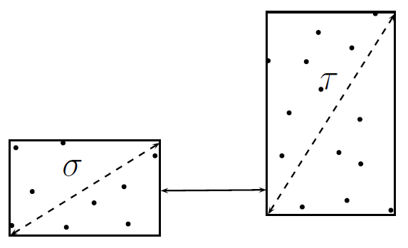
Admissibility.
ASERIS-BE implements various conditions including the well-known Hackbusch’s admissibility condition.
If clusters of DoFs \(\sigma\) and \(\tau\), of sizes \(m\) and \(n\) respectively, are admissible, then the interaction matrix block \(\mathbb{Z}_{\sigma, \tau}\) between them has a low-rank approximation:
where \(0 < \epsilon \ll 1\) represents a user-specified compression precision, \(U \in \mathbb C^{m \times r}\), \(V \in \mathbb C^{n \times r}\), and \(r \ll m, \, n\),
This is called an Rk matrix.
ASERIS-BE implements different compression methods allowing to recursively assemble \(U\) and \(V\), variants of Adaptive Cross Approximation method (ACA) enable performing this task on the fly without initially assembling the block.

Compression of a matrix block.
If the admissibility condition is not satisfied, and cluster sizes are larger than a threshold, the algorithm descend down the tree. At the leaf level, if the admissibility condition is not satisfied, a classical assembling is performed and the matrix block is stored as a full matrix block.
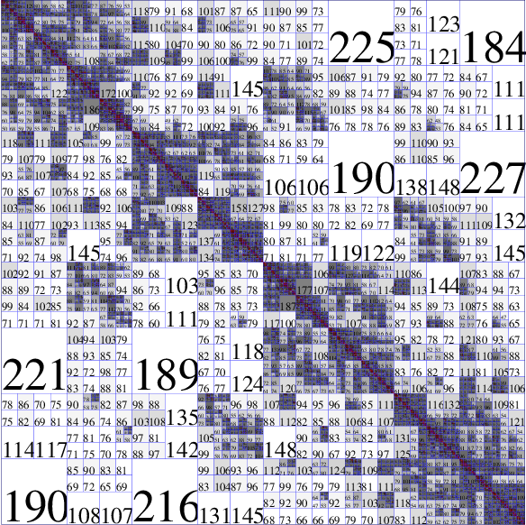
H-matrix block-cluster tree (with a non-symmetric assembly process) with the rank of Rk matrix blocks.
ASERIS-BE implements a complete solving procedure using H-matrix format. For example, using the Cholesky direct solver, matrix \(\mathbb Z\) is factorised: \(\mathbb{Z} = \mathbb{L}\mathbb{L}^T\) where \(\mathbb{L}\) is a lower triangular H-matrix. Solution of
is achieved by performing
ASERIS-BE solver is multi-RHS: \(\mathbb{U} \in \mathbb{C}^{N \times N_{\rm RHS}}\), here \(N_{\rm RHS}\) is the number of right-hand-sides. In this case \(I \in \mathbb{C}^{N \times N_{\rm RHS}}\).
Post-Processing
ASERIS-BE solver computes the (multi)vector \(I\) of the degrees of freedom, i.e. the fluxes across the mesh edges of the surface current densities.
Currents and charges
ASERIS-BE’s COUCHA postprocessing tool allows the computation the electric and magnetic currents and densities on the BEM mesh. This is done using the linear combination of the basis functions with the degrees of freedom as coefficients.
Fields and potentials
ASERIS-BE’s PROCHE postprocessing tool allows the computation of electric and magnetic near fields, potentials, as well as the Poynting vector at any position in the domain. This is done using the integral representations formulas with the computed currents.
Farfield
ASERIS-BE’s ANTEN postprocessing tool allows the computation of the farfield \(\mathcal{A} (\hat \xi)\) for any unit vector \(\hat \xi\), defined as
For example, when solving the EFIE (with only electric currents), it is written as

Spherical coordinates: far field direction \(\hat{\xi}\) as well as plane wave direction of arrival \(\hat{\nu}\) are defined by \((\theta, \phi)\) angles. Linear Vertical resp. Horizontal polarizations are defined as \(\hat{\theta}\) resp. \(\hat{\phi}\) components in the tangent plane.
Bibliography
L. Greengard and V. Rokhlin, “A fast algorithm for particle simulations”, Journal of Computational Physics, vol. 73, pp 325–348, 1987
G. Sylvand, “La Méthode Multipôle Rapide en Electromagnétisme: Performances, Parallélisation, Applications”, PhD thesis, École Nationale des Ponts et Chaussées, 2002
W. Hackbusch, “A Sparse Matrix Arithmetic Based on H-Matrices. Part I: Introduction to H-Matrices”, Computing 62, pp 89–108, 1999
W. Hackbusch and Boris. N. Khoromskij, “A Sparse H-Matrix Arithmetic”, Computing 64, pp 21–47, 2000
B. Lizé, “Fast direct solver for the boundary element method in electromagnetism and acoustics: H-Matrices. Parallelism and industrial applications”, PhD thesis, Université Sorbonne Paris Nord, 2014
K. Delamotte, “Une étude du rang du noyau de l’équation de Helmholtz : application des H-matrices à l’EFIE”, PhD thesis, Université Sorbonne Paris Nord, 2016