Lightning Indirect Effects
Description
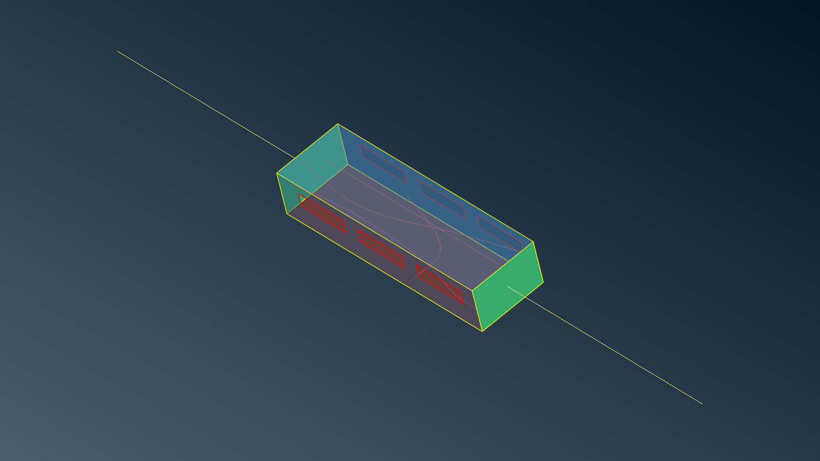
This case illustrates a Lightning Indirect Effect (LIE) problem. A “vehicle” with opened windows contains cables feeding some equipments. With the help of a wired channel outside the vehicle and some virtual junctions, a lightning path is defined.
We wish to compute the voltage on the equipments in the time domain for a A waveform excitation. The equipments are modelled using local values (local impedances).
Note
ASERIS-BE will compute the transfer function in the frequency domain. With the help of some Fourier post-processing tool we can easily come back to the time domain provided that the frequency sampling has been well chosen. The sampling is provided in a frequency file along with model.
Volumic domains
In this model there is only one homogeneous volumic domain, namely the unbounded freespace domain.
Surfacics domains
We consider a resistive surface CASE connected to two plies of PEC endings SIDES. The bottom of the casing is
a PEC GROUND.
Lineics domains
Two kind of wires are considered:
WIRES: wires supporting the equipments (inside)INJECTION: injection wires (outside)
The wires are connected to the casing.
The injection wires are connected to the PEC endings.
Local values
One local impedance (or port) is localized on each wire at the equipment position.
For the injection we consider a couple of so-called OUT local values. They have the following properties:
there must be 2
OUTlocal values in the modelthey must be localized at the free ends of the injection wires
the name must start with the keyword
OUT, e.g.:OUT_PORT_1andOUT_PORT_2
Finally a generator is placed on the injection wire next to the vehicle to actually provide the lightning excitation.
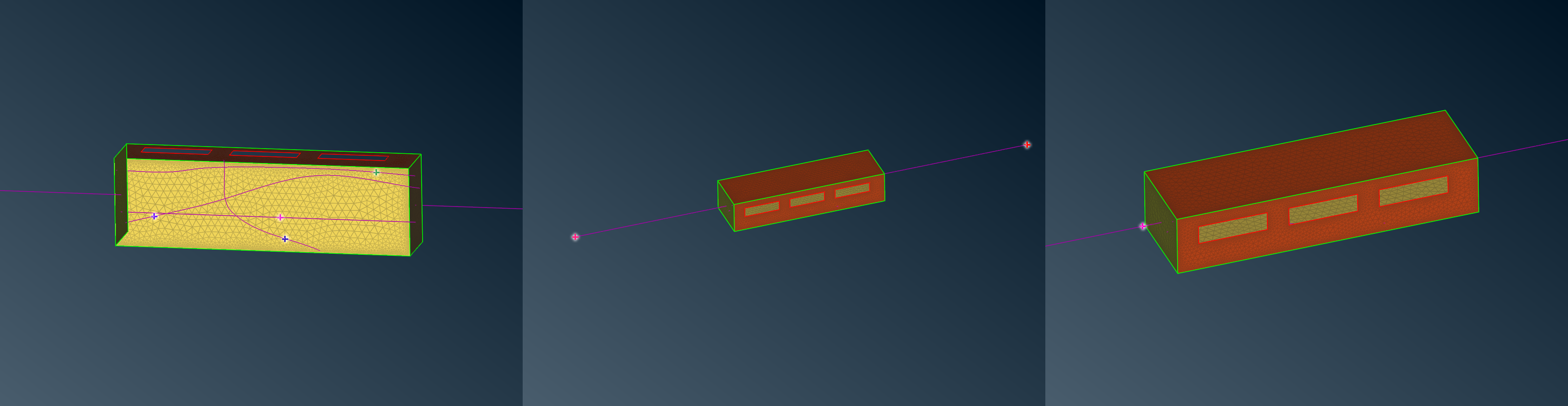
Position of local values: equipments (left), out (middle) and generator (right).
download
lie.zip (ansa v24.0.0)
CAD and mesh tips
Wires are meshed with NASTRAN CBEAM elements. Some assumptions must hold on the
lineic elements size and radius (see below) for the model to hold.
The spectrum of the A waveform (see Illumination) is such that we can consider frequencies from DC (1 Hz) up to 40 MHz.
The global mesh target is 30 cm, which is sufficient up to 100 MHz. Local refinement has been applied around free edges (windows) and sharp edges.
Note
With such frequencies we will need to use the low frequency stabilization option.
Simulation setup
Physical properties
The exterior volumic domain is naturally characterized by air properties \(\varepsilon=\varepsilon_0\) and \(\mu=\mu_0\), that is, relative permittivity and relative permeability of 1.0.
The resistive surfaces materials are characterized by:
Name |
Conductivity \(\sigma\) [S/m] |
Thickness \(d\) [m] |
Relative permittivity \(\varepsilon\) |
|---|---|---|---|
case |
1e5 |
0.003 |
\(\varepsilon_0\) |
ground |
1e7 |
0.002 |
\(\varepsilon_0\) |
The wires are characterized by:
Name |
Lineic impedance \(\rho\) [Ohm/m] |
Radius \(r\) [m] |
|---|---|---|
injection |
0.0 |
0.001 |
cable |
0.001 |
0.003 |
The local values of equipments are featured as passive impedances. They are defined according to their characteristics. The impedance of out local values is also a modelling parameter. For instance:
Name |
Impedance \(Z\) [Ohm] |
|---|---|
equipement 1 |
1e-3 |
equipement 2 |
4e-3 |
equipement 3 |
6e-3 |
equipement 4 |
1e-2 |
out |
1e3 |
The generator has no impedance and has a 1V e.m.f.
Illumination
The A waveform is the double exponential waveform defined by [1]:
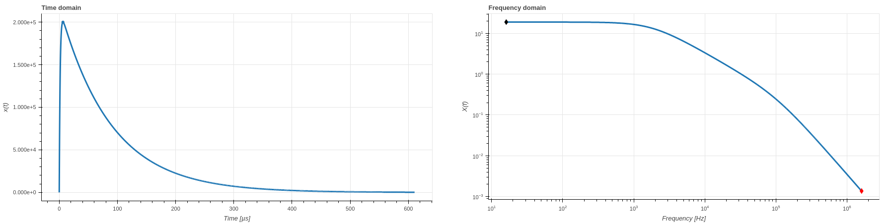
A waveform in time domain (left) and frequency domain (right).
For ASERIS-BE we will actually use a constant 1V generator to obtain a transfer function. Then some normalization will be applied to obtain the solution for such an excitation.
Observation
We look at the current on local values. Multiplying by the impedance provides the voltage.
Solver
For very low frequencies (\(\lambda > 100 \cdot \text{object diameter}\)) we can use the Eddy current approximation for faster computations.
Results
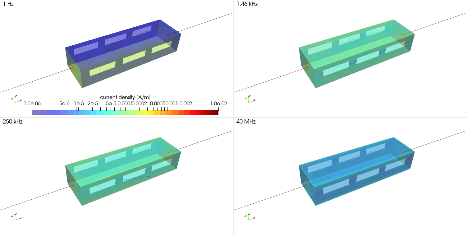
Current density for some frequencies and for 1V in the generator.
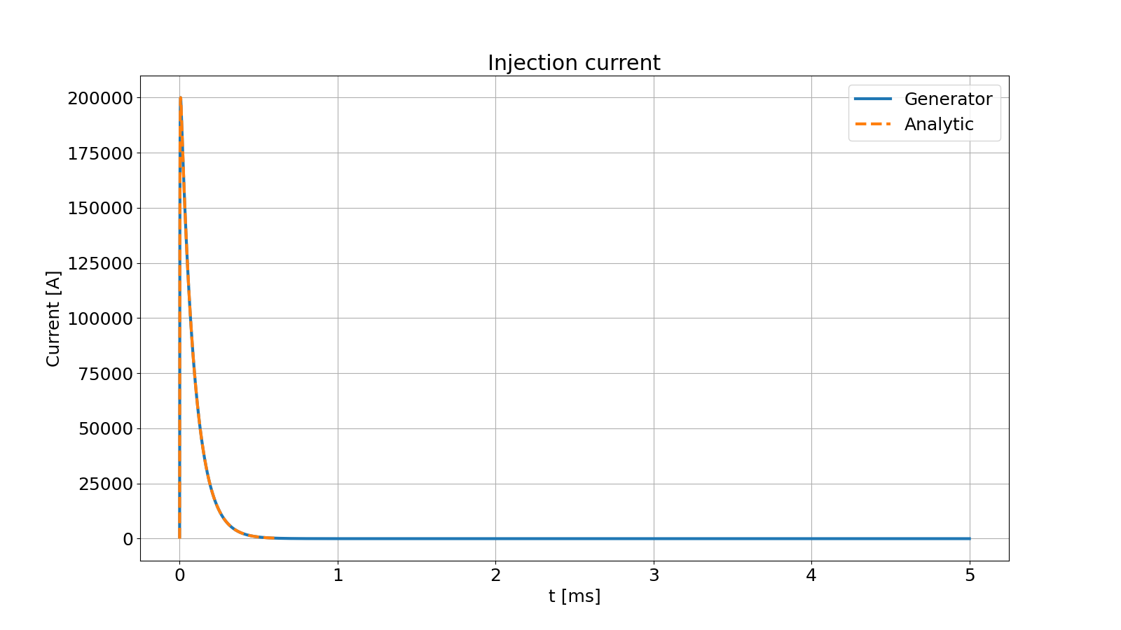
Injected current through the lightning channel. We can check numerically that the frequency sampling has been well defined: the time reconstructed waveform should match the analytical function.
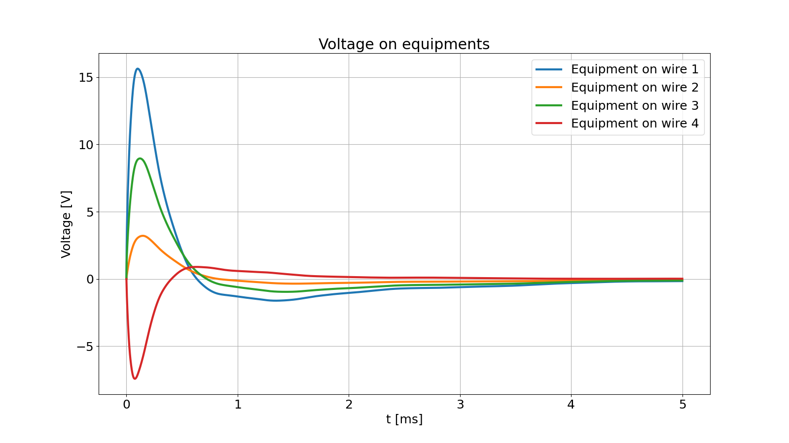
Voltage at equipments. Picks and time of rise are quantities of interest.