Horn
Description
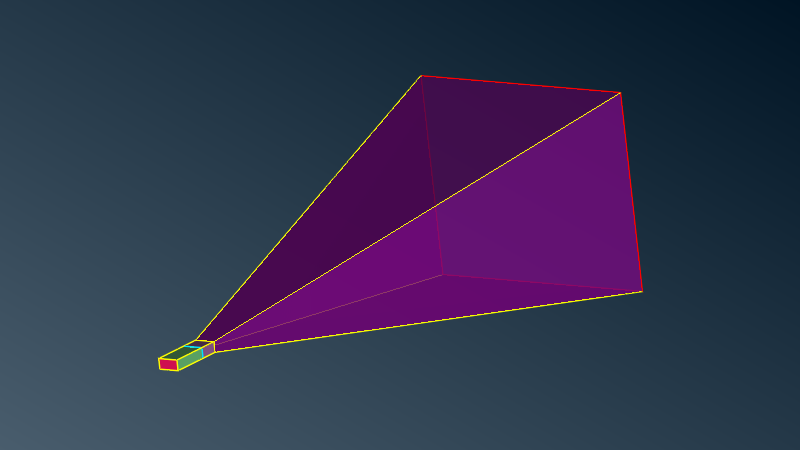
This model is made of a dielectric rectangular waveguide prolongated by a PEC (Perfect Electric Conductor) horn.
The basis section of the waveguide is a modal surface used to illuminate the wavegude with modes.
Note
Note that even if the waveguide was filled with air, ASERIS requires that its domain be considered as an independent closed domain.
We wish to compute the radiation pattern at 76 GHz for the \(\text{TE}_{10}\) propagating mode
download
horn.ansa.gz (ansa v24.0.0)
CAD and mesh tips
At 76 GHz the wavelength is about \(\lambda_0 = 4\) mm in the air and \(\lambda_d = 2.4\) mm in the waveguide.
We use a mesh length of \(\lambda_d / 20 = 0.12\) mm for the waveguide and \(\lambda_0 / 10 = 0.4\) mm at the horn extremities where the EM field varies the most. We can relax the mesh length to \(\lambda_0 / 5 = 0.80\) mm on the horn surface.
Note
This case is defined in millimeters.
Simulation setup
Physical properties
The exterior volumic domain is naturally characterized by air properties \(\varepsilon=\varepsilon_0\) and \(\mu=\mu_0\), that is, relative permittivity and relative permeability of 1.0.
The waveguide dielectric has relative permittivity \(\varepsilon_r=2.7\) and relative permeability \(\mu_r=1.0\).
Illumination
A rectangular waveguide can yield many Transverse Electric (TE) or Transverse Magnetic (TM) modes. Each mode is considered as a source and provides an independent solution. All solutions can then be recombined by linearity of the equations.
The modes that will be taken into account in the problem can be chosen:
using a threshold relative to the cut-off frequency (e.g. 110%)
selecting explicit modes with their index along the axes of the waveguide
Observation
The horn is pointing up towards (\(-\theta=45\) °, \(\phi=0\) °). We wish to compute the directive gain in the following window:
\(\theta_{min} = -90\) °, \(\theta_{max} = 90\) °, \(\Delta_\theta=0.2\) °.
\(\phi_{min} = 0\) °, \(\phi_{max} = 180\) °, \(\Delta_\phi=0.2\) °.
or on the whole sphere:
\(\theta_{min} = 0\) °, \(\theta_{max} = 180\) °, \(\Delta_\theta=0.2\) °.
\(\phi_{min} = 0\) °, \(\phi_{max} = 360\) °, \(\Delta_\phi=0.2\) °.
Solver
For such a large case select one of the fast solver: FMM or H-Matrix.
Use also the FMM acceleration for computing the far field diagram.
Results
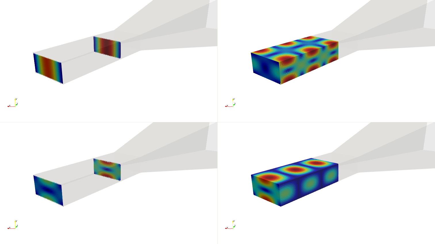
Propagating modes. One can visualize magnetic (left) or electric (right) current density for some of the modes on the modal surface: \(\text{TE}_{10}\) (top left), \(\text{TE}_{11}\) (top right), \(\text{TM}_{10}\) (bottom left), \(\text{TM}_{10}\) (bottom right). Magnetic current is visible only on the modal surface and at the dielectric interface at the other end of the waveguide since the casing is PEC.
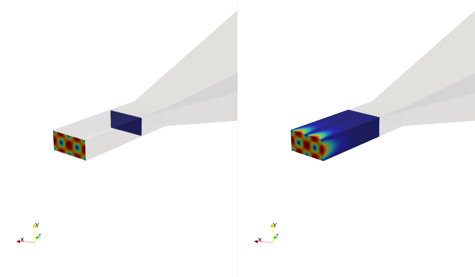
Evanescent modes. One can visualize magnetic (left) or electric (right) current density for the evenscent mode \(\text{TM}_{20}\). Note that the current has vanished at the end of the waveguide.
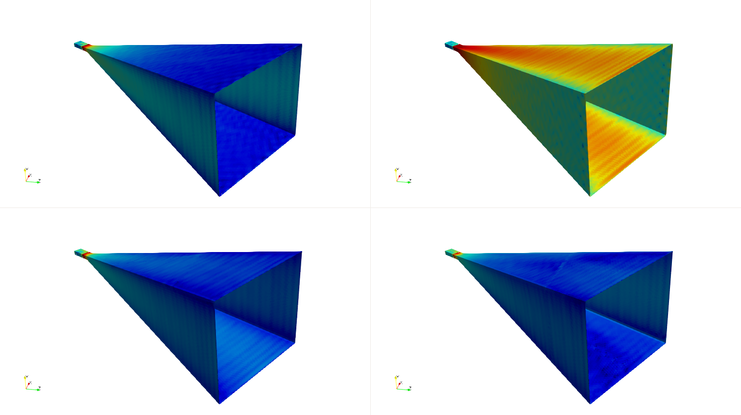
Current density inside the horn for the \(\text{TE}_{00}\) (top left), \(\text{TE}_{10}\) (top right), \(\text{TE}_{11}\) (bottom left) and \(\text{TM}_{10}\) (bottom right) incident modes.
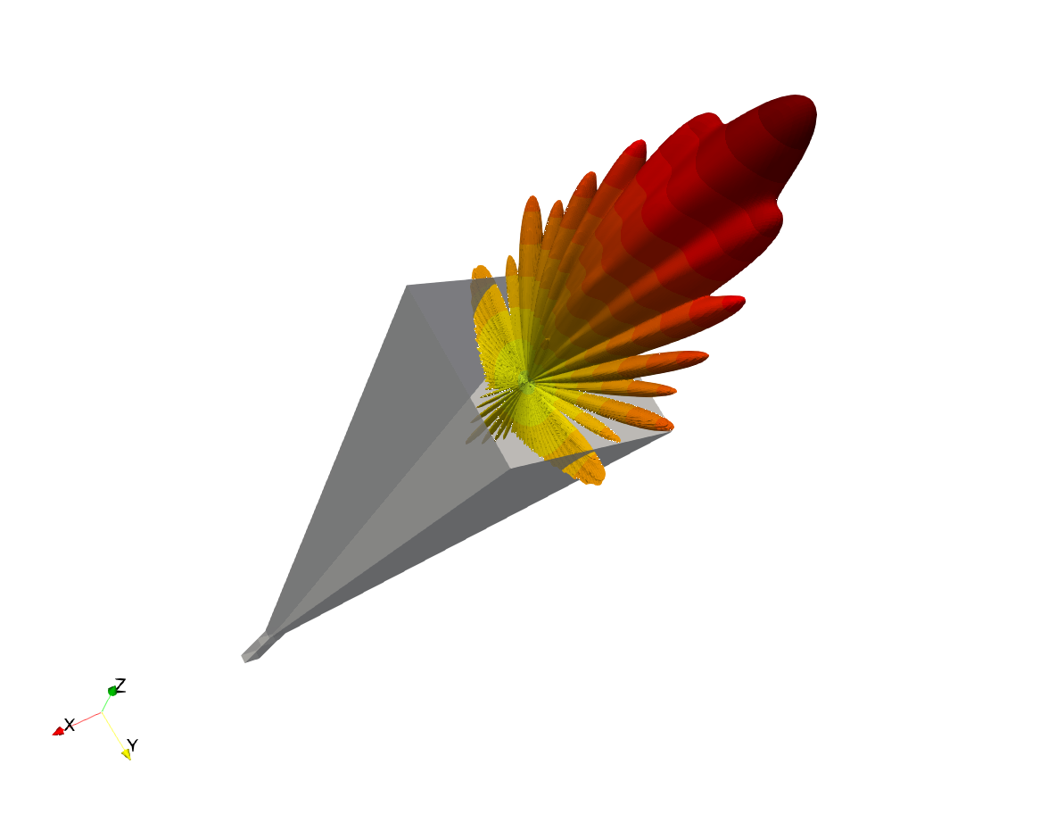
Far field directive gain pattern at horn exit.